Research log: PCB stepper motor
← Back to Kevin's homepagePublished: 2021 Dec 24I saw this sweet video of tiny magnets moving around a PCB:
and decided to replicate.
The SRI system consists of two main ideas:
- Generation of magnetic fields via PCB traces; think “unrolled bipolar stepper motor”.
- Diamagnetic (passive) levitation of magnets via a graphite layer between the PCB and magnets.
The first idea is interesting because it means cheap, precision-manufactured PCBs can be easily transformed into cheap, precise tiny motors.
The second idea is interesting because it removes “stiction” / mechanical hysteresis from the system; this allows the authors to demonstrate:
- ~1 um open-loop trajectory repeatability during levitation (compared to 15 um during sliding)
- 100 nm rms position repeatability
- using a photo-sensor to weigh a 140 ug grain of salt while a robot is moving at 1.5 cm/s
Seems pretty cool to me.
Prior art
Here’s all of the prior art I’ve found about these kinds of systems:
Ron Pelrine seems to have been investigating the broader topic since at least his 1988 PhD Magnetically levitated micro-robotics and appears to have led the SRI work:
- 2012 Diamagnetically Levitated Robots: An Approach to Massively Parallel Robotic Systems with Unusual Motion Properties introduces the magnets + PCBs + levitation graphite approach.
- 2013 patent on the technology.
- 2015 video shows more detailed robot motion along flex-PCBs.
- 2016 video shows self-assembly.
- 2016 Application of micro-robots for building carbon fiber trusses describes end-effectors built via chemically etching and bending 0.005 inch stainless steel; a 0.75 um sheet of pyrolytic graphite is used to reduce sliding friction, but isn’t sufficient to fully levitate the 5-magnet, ~10 mm robot.
- 2016 Optimal Control of Diamagnetically Levitated Milli Robots Using Automated Search Patterns describes searching for ideal control currents to minimize over/under-shoot when moving robots
- “In one test reported here, 150-μm moves were demonstrated at 90-nm rms error with 15-ms move times.”
- “currents for the four trace layers are [X1,X2,Y1,Y2] = [0.24, 0.28, 0.352, 0.4] A”
- 2017 Multi-Agent Systems Using Diamagnetic Micro Manipulation - From Floating Swarms to Mobile Sensors mostly overviews past work and describes how floating robots are cooler than other kinds of bearings
- “modulating the absolute magnitude of the traces increases or decreases the out-of-plane force between the board and the robot providing ~40–70 um Z-motion”
- 2019 Methods and Results for Rotation of Diamagnetic Robots Using Translational Designs describes methods for rotating robots.
- 2019 Nanoliter Fluid Handling for Microbiology Via Levitated Magnetic Microrobots describes using robots to stab hydrogel with pipettes; strangely it also has the most comprehensive mathematical treatment of the magnetic forces of any of the SRI papers.
- The circuit described uses PA74 op-amps ($90 dual package) on +/- 12V rails to convert a DAC input into precise current output
- 2020 Magnetic Milli-Robot Swarm Platform: A Safety Barrier Certificate Enabled, Low-Cost Test Bed describes a 12 x 12 matrix of independent zones driven by stacked H-bridges and four independent LM2673 buck converters acting as current sources (0.25 A, 0.3 A, 0.5 A, 0.7 A; presumably with higher currents for traces further from the surface); robots are a 5x5 array of 1.4 mm x 1.4 mm x 0.4mm N52 magnets; zone coordination and collision avoidance algorithms are also discussed.
Peter Misenko (Bobricus) implemented several versions; seeing his Hackaday writeup made the project seem more achievable for me as a hobbyist than the DARPA-funded SRI research papers:
- 2D stepper driver version using a L293 driver and 2 mm magnet, pushing 500 mA at 3V.
- MOSFET version 3 sets of unipolar-driven coils per dimension rather than 2 sets of bipolar (H-bridge) driven coils.
Miniatur Wunderland has been developing the technology for six years in an effort to build a 21 m long scale model of a Monaco Formula 1 race:
- 6-layer boards, traces 0.7mm apart
- cars have a 4-by-4 Halbach array
- hall-effect sensors are used to track car positions
Teeny Trains.com has their head in the same space.
SpritesMods.com was also inspired by the SRI video and built a simple board; however, they didn’t provide much detail about the current they needed to successfully move their magnets.
Jiří Vlček’s 2018 master thesis discusses simulations for various magnet, wire, and wire gap sizes and implements several PCB platforms:
- experimental currents are never reported, only the input voltage (~17 V) into their LN298P drivers (which will drop 3–5 V and go into thermal shutdown at higher currents).
- they do report the resistance of their coil traces, though; say 15 V after LN298’s drop; 45 Ohm coil would get about 330 mA and 5 Ohm coil would get whatever the LN298 can do at its thermal limit.
- the most PCB detail provided is “three layers layout” with 0.1 mm “layer gap height”; this could be achievable with a typical 4-layer board, using the top two layers for coil traces.
- Vlček’s supervisor is later involved in:
- 2020 Collective Planar Actuation of Miniature Magnetic Robots Towards Individual Robot Operation mentions 200 mA and 500 mA required to actuate a 1 mm x 0.5 mm disk magnet.
- 2020 Trade-off between resolution and frame rate of visual tracking of mini-robots on an experimental planar platform
Carl Bugeja’s YouTube channel has a lot of general experiments with (mostly rotary) PCB motors.
Planar Motors Inc. (founded 2017) has a very impressive industrial material handling system based on electronics-free, permanent magnet levitating platforms:
- research demo videos
- over-produced Acopos 6D presentation
- +/- 5 um positioning repeatability, 2 m/s speed, 0.5 – 4mm controllable levitation height, ability to weigh +/- 1 g
- “shuttle power consumption is about 15 to 50 W”
- The only patent application I could find relates to using the platforms in pick-and-place applications
Theory
The basic idea is to have two sets of serpentine coils and selectively run current through them to generate a moving magnetic field that drags along the permanent magnet “robot”. Consider this diagram from Vlček’s thesis; the robot consists of four permanent magnets glued to a square:
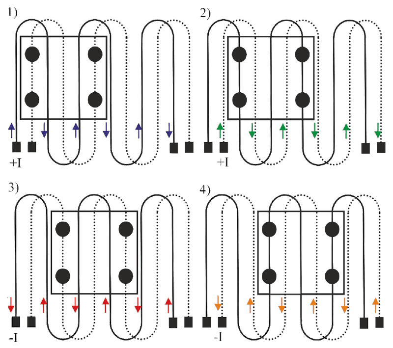
 When current is run through the first coil (blue), the leftmost pair of magnets are aligned with a magnetic field that’s going into the page.
Stopping the current on the first coil and starting it on the second (dotted, green) shifts the magnetic field to the right and the robot follows.
(Shout out to HyperPhysics for the right-hand-rule diagram, as well as helping me through undergrad.)
When current is run through the first coil (blue), the leftmost pair of magnets are aligned with a magnetic field that’s going into the page.
Stopping the current on the first coil and starting it on the second (dotted, green) shifts the magnetic field to the right and the robot follows.
(Shout out to HyperPhysics for the right-hand-rule diagram, as well as helping me through undergrad.)
When designing a PCB track, we can control:
- current
- coil width
- vertical distance between the coil plane and PCB surface
How do these factors relate the movement forces? We can estimate the force as the difference in energy between when the magnet is un-aligned with a coil (directly above a trace, position 1) and aligned (between two traces, position 2):
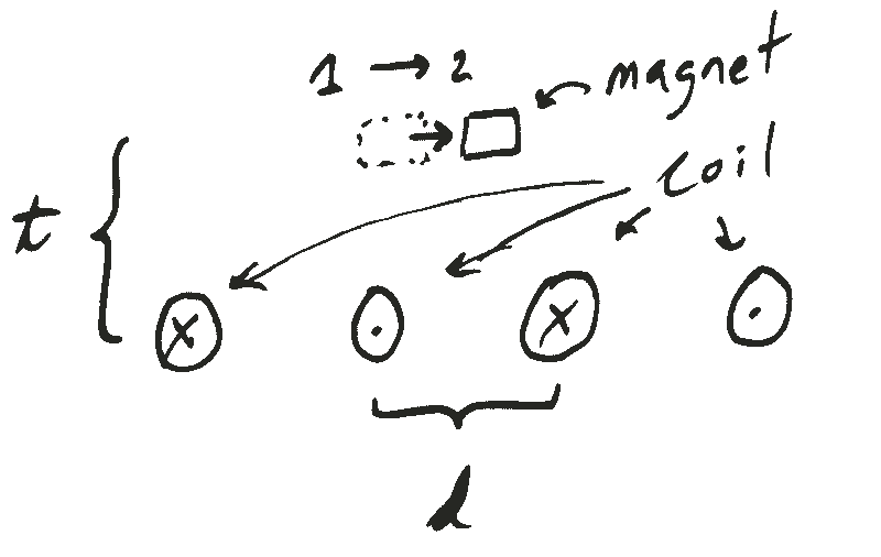
Furthermore, since the disk magnet is polarized through its axis, only the vertical component of the magnetic field contributes to the energy.
We can estimate using the equation for the magnetic field around infinite wire, where the field $B$ is proportional to the current $I$ over the radial distance $r$.
For position 1, first and third traces cancel each other out and the second trace contributes no vertical field component, which leaves just (in our approximation, anyway) the contribution of the fourth trace:
\begin{align} B &= I \frac{1}{\sqrt{t^2 + (2d)^2}} \newline B_\mbox{vertical} &= I \frac{2d}{t^2 + (2d)^2}. \end{align}
For the magnet on the same plane as the traces (t = 0), this agrees with the original equation, which suggests I did my geometry correctly: B = I / 2d.
For position 2, the first two wires give us vertical fields
\begin{align} B_{\mbox{vertical} 12} &= I \left( \frac{-3d/2}{t^2 + (3d/2)^2} + \frac{d/2}{t^2 + (d/2)^2} \right) \end{align}
and by symmetry the third and fourth traces will contribute the same vertical field as the first two, giving:
\begin{align} B_\mbox{vertical} &= I \left( \frac{-3d}{t^2 + (3d/2)^2} + \frac{d}{t^2 + (d/2)^2} \right) \end{align}
At t = 0 this reduces to:
\begin{align} &= I \left( \frac{-4}{3d} + \frac{4}{d} \right) \newline &= I \frac{8}{3d} \newline &= I \left( \frac{2}{d/2} - \frac{2}{3d/2} \right) \end{align}
which again agrees with the original equation. (I’m terrible at algebra, so I gotta keep re-checking…)
So in our 4-trace approximation, the energy difference — and hence the force — between the unaligned and aligned field positions is:
\begin{align} \Delta U &= I \left( \frac{2d}{t^2 + (2d)^2} - \frac{-3d}{t^2 + (3d/2)^2} - \frac{d}{t^2 + (d/2)^2} \right) \end{align}
I don’t have an intuition about this gross formula, but if we calculate some values around the dimensions of a 1 mm thick 4-layer PCB:
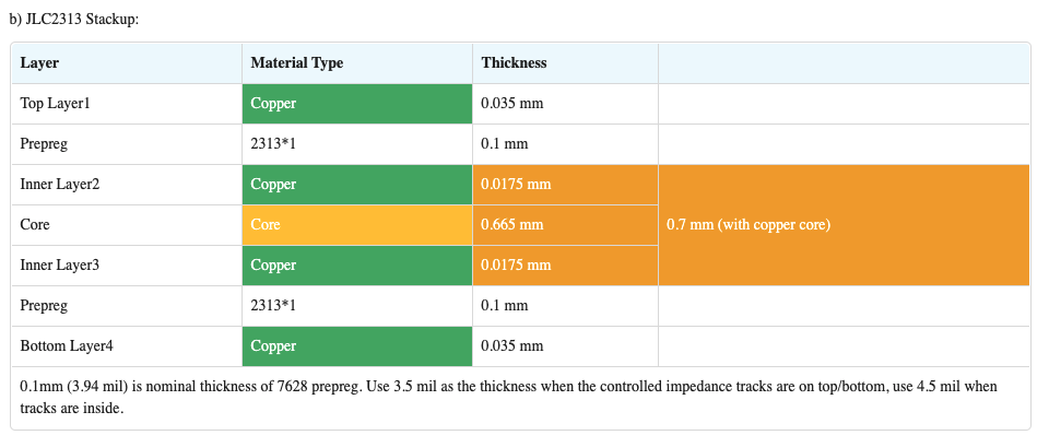
we get transition energies:
I was surprised to see that the transition energies become positive (i.e., the universe finds distasteful) at 0.6 and 1.2 mm for the 1 and 2 mm coil widths, respectively, suggesting that beyond those thicknesses we won’t be able to move magnets using coils on the reverse side of the PCB.
Take all these predictions with a grain of salt, and definitely drop me a line if you have an idea of how to model this with more fidelity than my high-school-algebra, 4-wire approximation =D
Initial proof of concept
Before designing a custom PCB I wanted to quickly establish viability, so I 3D-printed a template and hand-wound two serpentine coils (3 mm coil width / 1.5 mm trace-to-trace) of 30 AWG enameled magnet wire, covered with polyimide tape (for a smoother surface and to keep the wires from popping out), and drove with a tmc2209 stepper driver I had laying around at a 1.6 A current limit:
Here I’m using a 2 mm unrated neodymium magnet and triggering the steps manually. Later I got some 1 mm disk magnets from EBay where the seller at least listed them as N52, wound another template with 2 mm wide coils, and drove that programmatically:
I wasn’t able to drive these coils with drv8825 stepper drivers, even with the current-limiting potentiometer cranked entirely open. I suspect that the low resistance and inductance of the coil meant that it appeared as a short and triggered fault shutdown logic. (Though I wasn’t able to find anything in the datasheet about minimum motor coil inductance; once I got it working with the TMC driver I stopped looking.)
PCB v1 design
After the successful proof of concept, I set about designing a PCB. The requirements were:
- components available for assembly in JLCPCB’s catalog
- 5 V, 500mA max current target (suitable for driving via USB)
- separate zones to test 1 mm and 2 mm coil widths (0.5 mm and 1 mm step sizes, respectively).
- controllable via stm32f401 breakout boards
- a dozen or so levels of current control (something like 50 mA increments), just enough to play with micro-stepping and get a sense for power requirements
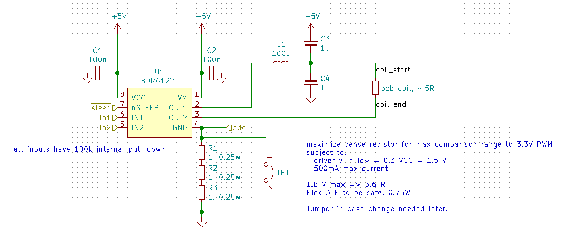
The rough idea was to modulate the current flow via PWM input to an H-bridge driver running the coil. Shout out to the folks on the EEVBlog forum who helped me resolve some of the issues with my initial approach. In particular, that the coils needed more inductance to slow current changes such that the average current could be modulated by a ~250 kHz signal, the max switching speed of the H-bridge.
(Think of a flipping a light switch: If the lights come on instantly, the room will always be fully bright or completely dark; but if the lights dim up/down at a rate much slower than you can flip the switch, you can adjust the room brightness to any level by flipping the switch back and forth.)
I wasn’t sure how to choose the actual values of the inductor and capacitors, so I modeled the circuit in Micro-Cap, a long-time commercial simulation software recently released as free. (Thanks, hope you are enjoying your retirement!)
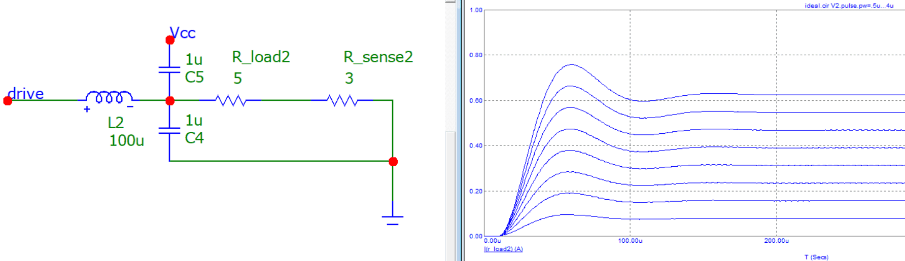
This diagram shows the current for pulse widths from 0.5 us to 4 us for a 250 kHz PWM signal; note that 4 us is the period of a 250 kHz signal, so the topmost current corresponds to a fully open switch and settles at the maximum steady state current of 5 V / 8 Ω = 625 mA.
There’s one H-bridge per coil, two coils per dimension, and two zones, so a total of 8 drivers. (Shout out to Mitja Nemec for their sweet replicate layout KiCAD plugin!)
For the coil patterns themselves I used KiCAD pcbnew’s Python API to generate plain traces and connected them manually to the respective drivers. This felt like a hack — the coils weren’t assigned to nets and would get eliminated by the “cleanup tracks and vias” tool — but I’m not sure what the “proper” solution is here; perhaps generating each zone (one side? both sides?) as a footprint and drawing the traces in there? I’m open to suggestions if anyone has ideas!
Anyway, I’m trying to avoid my tendency to get too precious with software, so I had a few drinks and just copy-pasted a lot of garbage Python loops, cleaned up manually, and put in my JLCPCB order on Dec 9 at 23:39. Five fully assembled, 0.8 mm thick, 2-layer PCBs were delivered to me in Seattle less than a week later, Dec 15 at 16:02; incredible.
PCB v1 evaluation
I got the PCB working:
which I always find to be a pleasant surprise =D
The 1 mm coils measure to about 8–9 Ω, which is pretty close to the 7 Ω estimate from KiCAD’s calculator for a 2.8 m, 0.2 mm wide 1 oz copper trace. (Take that number with a grain of salt; my \$20 multimeter reports 0.3 Ω when its leads are shorted and 3.4 Ω for the three 1 Ω ± 1% series sense resistors.) This gives us a max theoretical current of about 5 V / 12 Ω = 416 mA.
The 2 mm coils measure to 3.5 Ω so max current will be closer to 700 mA (or whatever Apple’s USB port decides to supply beyond the spec’s 500 mA).
However, switching frequencies anywhere close 250 kHz gave much lower currents than predicted. A 99% duty cycle gave for the 1 mm coil:
| freq (kHz) | current (mA) |
|---|---|
| 260 | 56 |
| 100 | 86 |
| 50 | 160 |
| 10 | 340 |
| 5 | 360 |
(Currents measured over sense resistors via the stm32f4’s ADC, readings taken 100x and averaged since the current is expected to be pretty choppy.)
I’m not sure how to explain this:
- H-bridge driver switching losses become substantial long before the rated 250 kHz PWM maximum?
- I setup the Micro-Cap simulation incorrectly by, e.g., failing to model MOSFETS and just assuming an ideal PWM voltage source?
It’s hard to say without looking at some waveforms, but my scope is still in Taiwan =(
For the “robots” I tested both single 1 mm diameter, 1 mm thickness N52 disk magnets and arrays of five such magnets press-fit into a resin-printed carrier, with the center magnet’s polarity opposite the outside four. This array could be reliably actuated at lower currents than the single magnet; the minimum was about 170 mA compared to 200 mA for the single free 1 mm disk magnet.
As for actuating via back-side coils, theory did in fact correspond to practice! I couldn’t get either single magnets nor the array to move on the 1 mm coil, but I was able to move a single magnet on the 2 mm coil.
For the 1 mm coil I even attached a higher voltage motor driver (drv8833, 10.5 V max motor voltage) and external power supply to push 1.1 A through the coils. I also ruled out the possibility the back-side coils were broken by flipping the board over; they work fine when they’re on the surface.
(Full disclosure: I designed the PCB and burned up a motor driver pushing current through the back-side coils before ever sitting down to do this writeup and the theoretical calculations above, so my algebra could be biased.)
The back-side 2 mm coils required full current to move the magnet reliably; about 600 mA compared to the 150 mA required by the top-side coils.
Next steps
With the basic hardware established, I see three directions for future work:
Levitation / sliding enhancements: I bought pyrolytic graphite from two sources, but neither clearly levitates my magnets. I’m not sure if my samples are substantially different than what SRI used; I have crystalline blocks and they they appear to use flexible sheet — perhaps like these intended for thermal applications? Both SRI and Miniatur Wunderland use Halbach arrays of thin square magnets rather than the disk magnets I’m using; perhaps that extra 4/π worth of magnet or the lack of free space between magnets makes all the difference to levitation?
I could also try improving sliding performance by treating the PCB surface with dry lubricant or drilling open vias / through holes and adding pressurized air to make a sort of air-hockey table (though I have no idea if the millimeter length scale skews more or less stable than the centimeter scale of an air-hockey puck).
I’d also need to figure out a protocol for measuring sliding friction — many repetitions of gently tilting a surface and measuring the angle when things slide off?
Control software: G-code interpreter, closed-loop computer-vision feedback system, zone synchronization (i.e., for a robot to traverse two v1 PCBs side-by-side, the coil phases must match up). There’s a lot to explore in particular if I get levitation working, as this now-expried Nikon patent notes:
As will be appreciated by those skilled in the art, many other commutations may be applied to the coils to achieve force and motion in the x, y, and z directions and torque and rotation about the x, y, and z axes.
Applications: Try and do something with the platform — sort grains of sand, self-moving tiny chess set, flight or ship tracker table top model, cheap precision x/y stage for super-resolution microscopy, some kind of clock/watch aesthetic complications, etc. In addition to refining the platform positioning and velocity accuracy, some applications may also entail designing and manufacturing end-effectors like cute lil’ robot arms or tiny cow catchers.
All of these directions will inform the next PCB design, which I expect will need to be 4-layers so the two coil layers are closer to the surface. It may also make sense in some cases to use more expensive 0.1 mm thick 2-layer flex circuits.